Two connected compact manifolds N and M are said to be bordant, if there exists a manifold W with boundary consisting of two connected components isomorphic to N and M respectively. The name comes from french and means sharing a boundary. Some people say cobordant, since the manifolds don't share a boundary but "are" shared as a boundary (I don't know how to explain this better than with the definition given above). We will stick to "bordant" because we investigate precisely what "the bordism of a manifold" and "the cobordism of a manifold" are.
One can see that being bordant is an equivalence relation, so it makes sense to speak of bordism classes of manifolds. By enriching N and M with extra structure (like a tangential framing, or an orientation), we get several different notions of bordism classes.
From each of these bordism theories, we get a sequence of spaces  such that is the Thom space of a universal bundle over some classifying space (I will explain that later) and
  is homotopy equivalent to
  . Homotopy theorists like to call such a sequence then a
The goal of this article is now to define Thom spectra and to give a geometric interpretation of the corresponding homology and cohomology theories, essentially by carrying out the Pontryagin-Thom construction relatively.
Preparation
Some Preliminaries on Transversality
To understand this article it may help to have seen the proof that framed cobordism  is isomorphic to stable homotopy groups of spheres, via the Pontryagin-Thom construction, but it is not strictly necessary.
I will assume some technical stuff on transversality, the most important being the
Theorem: Let  be a smooth map and
  a smooth codimension
  submanifold, such that
  intersects
  transversally (i.e. maps the tangent bundle of
  to a subbundle of the tangent space of
  that spans, together with the tangent bundle of , the whole tangent bundle of ), then the preimage
  is a smooth codimension submanifold of .
This theorem follows from the implicit function theorem much like the regular value theorem (by constructing appropriate coordinate charts), and generalizes it (take to be a point). It also generalizes the well-known constant rank theorem. To be transversal is a precise way of being "in general position".
The technical heart (in my opinion) of the Pontryagin-Thom construction (over a point) is the
Thom Transversality Theorem: Let be a smooth map and a smooth submanifold, then there exists an arbitraily small perturbation of (i.e. for any  a homotopic map
  such that the values are only varying in an
  -ball around each point) which is transversal to .
The transversality theorem roughly tells us, that being "in general position" is a generic property, which means that the exceptions are ... well, exceptional. This generalizes the theorems of Brown and Sard that tell us that regular values are dense, in the precise way that the transversal maps are a dense subset of the mapping space.
Spectra and (Co)homology theories
I'm assuming here that you already know the loop space functor. It assigns to a space  its space of (based) loops, topologized as subspace of the path space with the standard compact-open topology.
An  -spectrum
  is a sequence of spaces
  (indexed by natural numbers) with weak homotopy equivalences
  . Such objects generalize infinite loop spaces, since
  is an infinite loop space, and the extra contain additional information (the difference is precisely the question whether the spectrum is connective, but we won't need that in this article).
To each -spectrum one can associate a sequence of contravariant functors  by
by ![E^n(X) := [X,E_n]](https://www.konradvoelkel.com/wp-content/plugins/latex/cache/tex_fa9987f2788fba59dfb8baddf0a08ba7.gif) , the homotopy classes of maps from into the
, the homotopy classes of maps from into the  -th space of the spectrum. One can also associate a sequence of covariant functors
  by
by  , where
  is a spectrum with entries
  and the homotopy groups are defined as the homotopy groups of the
  -th space of the spectrum for non-negative, and there is a definition for negative that shouldn't bother us right now (for the connective spectra aka infinite loop spaces, the negative homotopy groups vanish anyway).
Now one can formally check that the covariant functors form a homology theory, while the contravariant functors form a cohomology theory (both in the sense of Eilenberg-Steenrod axioms), the only nontrivial thing to check is given by the fiber sequence resp. the cofiber sequence.
This term (summer 2012) I gave an expository talk on a theorem in the subject of stable homotopy theory:
Brown Representability Theorem: Every generalized Eilenberg-Steenrod cohomology theory is representable by a spectrum.
I have talk notes on infinite loop spaces, that cover the proof and the preliminary notions mentioned in this section more thoroughly (focusing on the cohomology side).
Classifying spaces
In what follows, we need to know what the classifying space  of the orthogonal group
  is. By definition, if there exists a contractible space with a free
  -action ( some topological group) then the quotient
  is called classifying space of , also denoted by
  .
.
For finite groups, this coincides with Eilenberg-Mac Lane spaces, but there is a considerable conceptual difference, which becomes visible for topological groups.
One has to prove that such a thing actually exists, and there are various constructions, notably the Bar construction. Instead of working in full generality, I just want to use a concrete model:
 , the infinite Grassmannian of -subspaces in some larger space. It is obtained as an inductive limit over the inclusions
 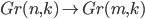 for
for  , where
  is the space of all -dimensional sub-vector spaces in
  .
.
There are inclusions 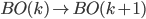 coming from inclusions
that are (in a certain sense) corresponding to inclusions  (both non-canonical, but easily fixed once and for all).
The contractible space with -action is given by the total space of the so-called tautological bundle, which is a vector bundle over that has as fiber over a point exactly the subspace of this point represents. This gives in the limit a vector bundle over  , with an obvious -action.
The terminology "classifying" comes from the fact that homotopy classes from a manifold into a classifying space for some topological group classify exactly the -principal bundles up to isomorphism. In particular, using the fact that the isomorphism classes of -principal bundles are in bijection with all vector bundles, we have
![[M,BO(k)] \simeq \{\text{rank } k \text{ vector bundles on } M\}](https://www.konradvoelkel.com/wp-content/plugins/latex/cache/tex_7258dec7f43c00154d1044bc2d6a6658.gif)
and the isomorphism is given by pulling back the tautological bundle along a map
 . That's why the tautological bundle is sometimes called universal bundle.
So it makes sense to take a codimension submanifold  , look at its normal bundle
  over
over  (which is of rank ) and assign to it a classifying map
  (actually only a homotopy class, but we can always choose representatives).
X-structures
We define X-structures, which allow an easy setup to define general Thom spectra later, out of the construction for BO (i.e. real vector bundles). If the X-business is too much for you, stick to X=BO. The following I learned from Switzer's book.
Definition: Let X be a sequence of spaces  together with maps
  and fibrations
  that commute with the canonical map
 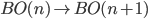 . An is a pair
  such that
  is an embedding with normal bundle classified by
 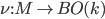 and
and  is a lifting of along the fibration
  .
.
An X-structure induces for all  maps
maps  and
and  .
.
Two X-structures  and
and  are called
  and a translation
  such that
  and
and  is homotopic to
  through liftings (i.e.
  commutes with the fibration
  for all times
  ).
).
An together with an equivalence class of X-structures.
The empty set will be regarded as n-manifold for all n, with unique X-structure.
If this X confuses you, you can take as concrete examples for  the cases
  (which yields framed (co)bordism, as studied by Pontryagin) and
  (which yields ordinary (co)bordism).
Definition: A  between manifolds with X-structures and
  such that there is a translation
  with
with  and there exists a homotopy
  that lifts
  .
.
Definition: Let  be two closed n-dimensional X-manifolds. They are called
  , if there exist (n+1)-dimensional compact X-manifolds
  such that
  are X-diffeomorphic (with the induced X-structures on the boundaries).
This is easily seen to be an equivalence relation, we write  or
or  for the classes. One can also show that disjoint union gives an abelian group structure with
  as neutral element.
Thom spectra (for X-structures)
Now we're going to construct the objects I want to investigate. For a general first idea what Thom spaces are about, you can have a look at my previous post on Thom spaces and their interpretation as twisted suspensions.
Definition: Let  be a rank n vector bundle. Taking any inner product on the fibers, we can consider
  an
an  -bundle and thus define the disk bundle
  and the sphere bundle
  . Taking the quotient of the total spaces yields the

which comes with a natural projection
 .
.
If the base of a bundle has a CW structure, so has the Thom space (and one can describe the structure precisely).
The Thom construction extends to maps, since any map of -bundles  satisfies
  and
and  , so we have

Proposition: For vector bundles over and  over
over  , there is a natural homeomorphism

This is essentially the homeomorphism

As a corollary, look at
 as
as  with
with  a trivial bundle (first regarded over the same space as but then as bundle over a point), then we have
Definition: Let  be an X-structure and denote by
  the universal (tautological) -bundle over
  . Pulling it back to X we have
  , which satisfies

so
induces a bundle map  and on Thom spaces
This is the data for a spectrum
 and it is customary to use the notation
  for the -spectrum (to calculate homotopy groups), one still needs to stabilize, i.e. take
  . We will not do this, but rather represent a homotopy class in
  by a map
  for some very large , which amounts to the same.
Let's see what we've got so far: we have defined various spectra associated to X-structures. We also have a notion of being X-cobordant. The following will bring these threads together.
Thom's theorem and (co)bordism (co)homology
Thom's theorem over a point
Theorem:  .
.
Proof:
We first describe a map  defined on the X-diffeomorphism classes of X-manifolds of dimension n into
  , then we show that it factors through a homomorphism
  . This map is shown to be surjective and with similar arguments, that it is also injective.
Given a closed smooth n-dimensional manifold with X-structure , where , we regard  as the 1-point compactification of
  and the normal disk bundle
  of in as a tubular neighbourhood of in
  . We define a map
  (which represents a homotopy class of the Thom space of ) by letting it be the projection
  on the subset
  and the constant map to the basepoint on the complement. This is continuous since the boundary of is also sent to the basepoint by construction. By composing with
  we get a map
  , thus a map of spectra
  and define
 ![\Phi(M):=[f_M] \in \pi_n(MX)](https://www.konradvoelkel.com/wp-content/plugins/latex/cache/tex_c81bc09bd9f2f44a72ca67120a0c26a8.gif) .
.
Now we show that the disjoint union of two n-dimensional X-manifolds  is mapped by to the sum
  .
.
We may assume  in by translating the map
  away from the image of
  (by virtue of the definition of an X-structure, this still gives the same X-structure). We can even translate and such that one lands entirely in the upper half space and the other in the opposite half space, so that we observe that
  is
is  on the upper hemisphere and
  on the lower hemisphere. The map
  thus factors through
  , by pinching the equator of
  to a point.
The next step is to show that is invariant under X-cobordism. Let  be an X-manifold with boundary, where we regard
  after translation as embedding into
  and thus as embedding into
  , with
  landing in
  . Again we proceed to obtain a map
  that yields a map
  which is a homotopy from
  to
to  , so we observe
 ![[f_{\partial W}] = 0 \in \pi_n(MX)](https://www.konradvoelkel.com/wp-content/plugins/latex/cache/tex_6c1ee97b232dcd2211316b5526253d7d.gif) .
.
In particular, two X-manifolds that are X-cobordant  via some X-manifold
  with boundary
  yield
yield ![[f_M] - [f_{M'}] = [f_{\partial W}]](https://www.konradvoelkel.com/wp-content/plugins/latex/cache/tex_a99a966d7a067a78a8090aa6ee7ba1cb.gif) , so we have
, so we have ![[f_M] = [f_{M'}]](https://www.konradvoelkel.com/wp-content/plugins/latex/cache/tex_37ae20986069485e5d72a11eb516d82d.gif) and thus factors through a homomorphism .
and thus factors through a homomorphism .
For surjectivity of we take a map  representing a class in
  and construct an X-manifold as codimension submanifold of such that
  , i.e.
 ![\Phi(M) = [f] \in \pi_n(MX)](https://www.konradvoelkel.com/wp-content/plugins/latex/cache/tex_3fd15ea527b90931d16fb5b76c7f0983.gif) .
.
To do that, we slightly deform  such that it is transversal to , which allows to take
  . The homotopy can be lifted to a homotopy of , since
  was required to be a fibration. Taking a tubular neighbourhood of inside
  we can carry out the same argument, taken to be transversal to and so we get
  as a tubular neighbourhood of . This gives us an X-structure on and at the same time we can see that the map assigned by to is homotopic to .
Injectivity uses the same transversality trick that we just saw. Take two manifolds  with
with ![[f_M] = [f_{M'}] \in \pi_n(MX)](https://www.konradvoelkel.com/wp-content/plugins/latex/cache/tex_447a38730c1f8e1f7b99ac18a20bcc85.gif) , so we have a homotopy
, so we have a homotopy  with
with  and
and  . With the transversality trick we deform
  such that
  is a submanifold. It is necessarily a dimension n+1 submanifold, since each
  is a codimension k submanifold of
  . We see that and with the tubular neighbourhood trick we get an X-structure on W as well.
Singular manifolds, relative Thom's theorem
Now that we understood the situation over a point, the general case will not be much harder. I will briefly state what we do now:
To any spectrum one can not only associate it's homotopy groups but also a (reduced) homology functor  . We will write
  and call it the k-th X-bordism of . The question is: what is the (geometric) meaning of the k-th X-bordism of some manifold?
The answer is, that the k-th X-bordism of classifies the , up to cobordism. The case of  was solved in the previous subsection, where "singular X-manifold over a point" reduces to "X-manifold".
Definition: A continuous map  from a closed X-manifold to is called . Two singular X-manifolds ,
  are with boundary
  together with a continuous map
  that restricts to the singular X-manifolds
  ,
,  .
.
Theorem: 
Proof:
The strategy is the same as in the previous proof. First I summarize, then we can go through the details:
a) To each compact smooth n-fold (with an X-structure) with continous map  we assign a map
  by the Thom space construction (here, one does something different than in the case ).
b) We compose such a map  with the projection
  and also with
  (order doesn't matter), and take homotopy classes. We obtain a map that factors through X-diffeomorphisms

c) Show that disjoint union of manifolds corresponds to addition in the homotopy group, by the pinching trick (putting one manifold in the upper and the other in the lower hemisphere).
d)
factors through a group homomorphism  , since an X-cobordism of singular manifolds and
  yields a homotopy
  between and
  .
.e) Surjectivity of
is done with the transversality trick: We get a preimage of some ![[f]](https://www.konradvoelkel.com/wp-content/plugins/latex/cache/tex_7b93cec8a8b3e110392556212941efcd.gif) by taking a representative that is transversal to
by taking a representative that is transversal to  , and then
  is a manifold with continuous map
  such that
  .
.f) Injectivity also uses the transversality trick: For two singular X-manifolds
 that get mapped to the same homotopy class, we have a homotopy between and that comes from a cobordism (essentially by surjectivity of some kind of ).
The difficulties lie in step a) and that one has to keep track of the "singular" thing, i.e. we don't have just manifolds on the left hand side, but continuous maps.
So I explain step a) in more detail now:
Let be a singular X-manifold. Consider the (n+k)-sphere as one-point compactification  and define
  by
by  , where is the map induced by the X-structure and
  is the composition
  that assigns to each vector in the normal bundle the image of its footpoint under
  . On the complement, we send everything to the basepoint,
  . We compose the result with the contraction
 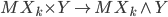 . That's the map . The assignment
  is well-defined on the level of X-diffeomorphism classes of singular X-manifolds, and we call this map .
Change of coefficients: Bockstein
Every complex manifold has a complex normal bundle, so it comes with a  -structure (X is now
  ). This means that we can look at
  by forgetting this extra structure. At the same time we can look at as inducing a map of spectra
  that induces homology morphisms
  , that coincide with the map described before.
One can now ask whether two non-complex-cobordant manifolds become real-cobordant, i.e. whether their images under the Bockstein morphism just sketched coincide. One can also ask whether a given real manifold is in the image of the Bockstein morphism.
The new thing is now, that we can use fiber sequence technology to get more information. Since is required to be a fibration, we can call the fiber  and get a long exact sequence

The connecting morphism in this long exact sequence is sometimes the only one called "Bockstein".
Cobordism Cohomology
I wanted to discuss this in more detail, but then I got exhausted from writing up, so here is a rough sketch:
Cobordism Cohomology can be defined as ![MX^n(Y) := [S^k \wedge Y, MX_{n+k}]](https://www.konradvoelkel.com/wp-content/plugins/latex/cache/tex_fb809ab8feb72b607eb921e13b6ca261.gif) for large enough. One can try to do the same as for homology, to identify the "geometric" object
for large enough. One can try to do the same as for homology, to identify the "geometric" object  should be isomorphic to: Given a homotopy class
 ![[f] \in [S^k \wedge Y, MX_{n+k}]](https://www.konradvoelkel.com/wp-content/plugins/latex/cache/tex_563bf91c914400a32a57eda0176e21aa.gif) , we can choose a representative that extends to
, we can choose a representative that extends to 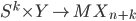 such that it's transversal to
  in
in  and then
  is a smooth submanifold of
  which becomes a singular X-manifold in by projecting to . Working out the dimensions, we get
  .
.
For a better overview in the special case  you can look at Atiyah: Bordism and Cobordism.
Outlook
There are various things one can do from this point on.
- Do the same stuff algebraically, as in Morel-Levine's book on algebraic cobordism.
- Look at framed cobordism to get some knowledge about stable homotopy groups of spheres (Pontryagin's observation)
- Look at complex cobordism and the Adams-Novikov spectral sequence to get even more knowledge of stable homotopy groups. This is currently discussed in a rather long series of blog posts by Akhil Mathew.
- Use a better understanding of cobordisms to get some knowledge about mapping class groups, as in Madsen-Weiss.
- Forget all this stuff (maybe you didn't read it carefully in the first place, so why bother?)


Comments
Dear Dr. Voelkel
I learned many things from your pretty note on "Bordism
and Cobordism". I just want to know the precise title
of th "Switzer's book" that you have referenced in the text.
Sincerely yours,
Sahand Raman
(... not a Dr. yet ...)
Switzer's book is called "Algebraic Topology: Homotopy and Homology".