This post is the continuation of "From the Langlands Correspondence for Function Fields to the Geometric Langlands Correspondence I", and explains how to translate the Langlands Correspondence for function fields to a geometric question.

This post grew out of the preparation for a seminar talk on this topic and is separated in two parts, this being the second, and last part.

To repeat briefly, the Langlands Correspondence for a function field $F = \mathbb{F}_q(X)$ of a smooth projective curve $X$ states that certain n-dimensional irreducible l-adic Galois representations correspond (1:1) to irreducible cuspidal automorphic representations of $GL_n(\mathbb{A}_F)$. Furthermore, the L-functions of Galois representations and automorphic representations coincide.

Translation of the Galois side to Geometry

"Galois groups are fundamental groups"

Think about étale fundamental groups of schemes, and observe that the étale fundamental group of the spectrum of a field is just the Galois group of the maximal unramified extension (i.e. the seperable hull of the field) over the field. Hartshorne even defines the "algebraic fundamental group" of a curve this way.

Look at field extensions of $\mathbb{C}(t)$ and their 1:1-correspondence to (ramified) covering spaces of $\mathbb{P}^1$ (up to birational equivalence). The Galois correspondence tells us that field extensions are classified by the Galois group, and basic homotopy theory tells us that covering spaces are classified by the fundamental group. The Galois group can only see finite extensions and their limits, so it is a profinite group. The fundamental group isn't, but its profinite completion is isomorphic to the Galois group.

Imagine $\mathbb{C}^\times$, the complex plane with removed origin. Vector bundles on this space carry a natural monodromy operation, which is: take a local (constant) section and move it along transition maps of a trivializing cover of the bundle around the origin, back to the open set where it came from. You'll end up with some section, but not always with the section you started with. The difference (or should I say quotient?) on a fibre is given by a linear map, the composition of the transition maps you used to transport around the origin. This linear map is called the monodromy, and it can be shown that it doesn't depend on the concrete path, but only on the homotopy class of the path you chose around the origin. This gives rise to a representation 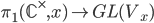$\pi_1(\mathbb{C}^\times,x) \to GL(V_x)$, where $V_x$ is the fiber over the basepoint $x$, where you started the whole thing.
This monodromy representation actually exists for every space, with any basepoint, and every vector bundle on it.

Given a finite field $\mathbb{F}_q$, the Galois group look similar to the fundamental group of 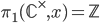$\mathbb{C}^\times$, since $\pi_1(\mathbb{C}^\times,x) = \mathbb{Z}$ and $Gal(\overline{\mathbb{F}_q}/\mathbb{F}_q) = \hat{\mathbb{Z}}$, the profinite completion. The finite extensions of $\mathbb{F}_q$ are the fields $\mathbb{F}_{q^n}$ and each such extension consists of adjoining roots of unity, so it is correct to picture $\mathbb{F}_q$ and its extensions as a circle of roots of unity. The Frobenius element $x \mapsto x^q$ of $Gal(\overline{\mathbb{F}_q}/\mathbb{F}_q)$ serves as substitute of "going around the circle once" (and it is a topological generator of the Galois group).

That should be enough for motivational purposes so far, I'll end with a theorem:
On a smooth projective curve $X$ defined over a number field $K$ (or the rationals, or the integers), the étale fundamental group is the profinite completion of the topological fundamental group of the analytified space $X^{an}$ for some embedding $K \hookrightarrow \mathbb{C}$.

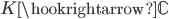"Monodromy representations are local systems"

A local system on a space $X$ is a locally constant sheaf of finite dimensional vector spaces. As just explained, it admits a monodromy representation on the fiber over any point. We will now see how to reconstruct a locally constant sheaf from its monodromy representation and hence establish a bijection between representations $\pi_1(X,x) \to GL_n(\mathbb{C})$ and local systems, up to isomorphism:

Let $(\tilde{X},\tilde{x})$ be the basepointed universal covering space of $(X,x)$, then $\pi_1(X,x)$ acts on it, with quotient $X$. Given a representation 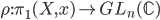$\rho : \pi_1(X,x) \to GL_n(\mathbb{C})$ we define a local system as quotient of the trivial local system on $\tilde{X}$:

$$\tilde{X} \times_{\pi_1(X,x)} \mathbb{C}^n := \left\{ (\tilde{y},v) \in \tilde{X}\times \mathbb{C}^n \right\}/(\tilde{y},v)\sim (g\tilde{y},\rho(g)v),\ g \in \pi_1(X,x).$$

So we replace certain l-adic Galois representations with certain l-adic local systems. Here, l-adic local system means that the fibers are $\mathbb{Q}_\ell$-vector spaces. The ramification condition on the Galois side is translated into the condition that the local systems are defined over the complement of finitely many points, called the ramification points, and satisfy a condition called "regular singularities" on these points.

For a complex curve $X$ we can also look at local systems of $\mathbb{C}$-vector spaces, corresponding to representations of the topological fundamental group.

Translation of the Automorphic side to Geometry

Now we're going to translate the cuspidal automorphic representations into something more geometric, though we will have to restrict to unramified automorphic representations (otherwise it's quite complicated).

We will do this in several steps: First I'm going to give you a bijection of cuspidal automorphic representations with certain cuspidal automorphic functions, then I give the space where these are defined a new (algebraic) structure (the moduli stack of vector bundles) and then discuss the general function-sheaf correspondence, which can finally be applied to replace the cuspidal automorphic representations with certain sheaves on the moduli stack of vector bundles, more precisely the Hecke eigensheaves (which are not sheaves, but perverse sheaves). In the end, I don't want to go into much detail, especially I don't want to explain what l-adic sheaves or perverse sheaves are.

From automorphic representations to automorphic functions

A cuspidal automorphic representation 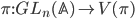$\pi : GL_n(\mathbb{A}) \to V(\pi)$, which is by definition an irreducible subrepresentation of the right action of $GL_n(\mathbb{A})$ on the space of all locally constant, K-finite, cuspidal functions, with central character, on the quotient 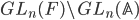$GL_n(F)\backslash GL_n(\mathbb{A})$. We have the tensor product description of $\pi$ by local representations: $\pi = \otimes \pi_x$. By definition, this $\pi$ is unramified at a place $x \in X$ if $\pi_x$ is unramified, which by definition means that the invariants $V(\pi_x)^{GL_n(\mathcal{O}_x)}$ are not the zero vector space. From irreducibility of $\pi_x$ we can see that these invariants are an irreducible module for the spherical Hecke algebra $\mathcal{H}_x$, which is an abelian algebra, hence its irreducible modules must be one-dimensional. This in turn implies we get a vector 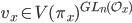$v_x \in V(\pi_x)^{GL_n(\mathcal{O}_x)}$, unique up to scalar, and thus a function 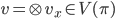$v = \otimes v_x \in V(\pi)$. The space of all translates of this vector $v$ under $GL_n(\mathbb{A})$ is an irreducible subrepresentation of $\pi$ and as such coincides with $\pi$, so $v$ determines $\pi$ uniquely.
As a last remark about this situation, $v$ gives rise to a function on the double quotient

$$f_\pi : (GL_n(F) \backslash GL_n(\mathbb{A})) / GL_n(\mathcal{O}) \to \mathbb{C}$$

We have just established a correspondence

$$\{\text{cusp. auto. rep. } \pi \} \leftrightarrow \{\text{lc cusp. cent.char. } GL_n(F) \backslash GL_n(\mathbb{A})/GL_n(\mathcal{O}) \to \mathbb{C}\}$$

The moduli space of vector bundles as adelic double quotient

Starting slowly, take a line bundle $L$ over the curve $X$, say in the analytic topology if $X$ is defined over the complex numbers (where it is easy to draw pictures). If you need a more severe headache, think of the Zariski topology instead and define your curve over an arbitrary field $k$, it will not make a big difference.

This line bundle trivializes over some open set, by definition. In the Zariski topology, open sets on a curve are just the complement of a finite set of points, which we want to call $S \subset X$, so $L$ is trivial over $X \setminus S$. In the analytic topology, there is some work necessary to find a finite set of points such that the line bundle is trivial over the curve, but it can be done by finding a not-everywhere-vanishing meromorphic section $s$ of the line bundle and setting $S := supp(div(s))$, the set of poles and zeroes of $s$. To find a meromorphic section, the best way I know of is to use a theorem of Serre which gives a holomorphic section $s\cdot z^n$ for some twisted bundle $L(n)$, which generates $L(n)$. There you also need to understand that a trivialization is quite the same as a nowhere vanishing holomorphic section.

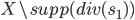If you take a vector bundle $E$ of rank $n$, you can do the same tricks to get a meromorphic section $s_1$ of $E$, so over $X \setminus supp(div(s_1))$ the section $s_1$ is a holomorphic section and thus spans a rank 1 sub-bundle of $E$. By quotienting out this sub-bundle, we get a rank $n-1$ vector bundle on $X \setminus supp(div(s_1))$ and can do the same trickery $n-1$ times more, until we have 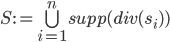$S := \bigcup_{i=1}^n supp(div(s_i))$ and over $X \setminus S$ holomorphic sections $s_1,...,s_n$ which are even linearly independent, so $E$ is trivial over $X \setminus S$ by these sections.

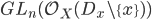
If you take a point $x \in S$, you can find a small open subset of $X$ such that $E$ trivializes over this subset (again, by definition of a vector bundle). In the analytic case, you can take a small disc (and draw that picture in your mind even in the general case), and hence call such a chosen open subset $D_x$. We want to choose $D_x$ such that it contains no points of $S$ except $x$ itself. The line bundle is now completely described by the trivialization over $X \setminus S$ and the trivializations over each $D_x$ and the transition functions on the intersections $D_x \setminus \{x\}$. These transition functions are holomorphic functions

$$D_x \setminus \{x\} \to GL_n(k)$$

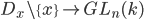
so we can think of them as elements of $GL_n(\mathcal{O}_X(D_x \setminus \{x\}))$.

We have just established a correspondence

$$\prod_{x \in S} GL_n(\mathcal{O}_X(D_x \setminus \{x\})) \leftrightarrow \{\text{rank n vector bundles with fixed trivialization over } X\setminus S \text{ and all } D_x\}/\simeq.$$

If we change the trivialization over $X\setminus S$, this amount to multiplying the transition functions from the left by a holomorphic function on $X\setminus S$, so in our presentation by an element of $GL_n(\mathcal{O}_X(X\setminus S))$ and we get the correspondence

$$GL_n(\mathcal{O}_X(X\setminus S)) \backslash \left(\prod_{x \in S} GL_n(\mathcal{O}_X(D_x \setminus \{x\}))\right) \leftrightarrow \{\text{rank n vb w/ fixed triv. over all } D_x, \text{ which are trivial over } X\setminus S\}/\simeq.$$

Doing the same thing with changing trivializations on the $D_x$ is clearly possible and we can furthermore add product factors on both side of the quotient without changing it to get the correspondence

$$\small GL_n(\mathcal{O}_X(X\setminus S)) \backslash \left(\prod_{x \in S} GL_n(\mathcal{O}_X(D_x \setminus \{x\})) \times \prod_{x \in X\setminus S} GL_n(\mathcal{O}_{X,x})\right) / \left( \prod_{x \in S} GL_n(\mathcal{O}_X(D_x)) \times \prod_{x \in X\setminus S} GL_n(\mathcal{O}_{X,x})\right)$$

$$\leftrightarrow \{\text{rank n vb which are trivial over } X\setminus S \text{ and all } D_x\}/\simeq.$$

Now we want to take smaller and smaller open sets $D_x$ and in the inductive limit the sheaf $\mathcal{O}_X$ gives us $\lim_{\rightarrow} \mathcal{O}_X(D_x) = \mathcal{O}_{X,x}$, the stalk, and $\lim_{\rightarrow} \mathcal{O}_X(D_x \setminus \{x\}) = \mathcal{M}_{X,x}$, the stalk of meromorphic functions. I want to introduce the $S$-Adèles now:

$$\mathbb{A}(S) := \prod_{x \in S} F_x \times \prod_{x \in X\setminus S} \mathcal{O}_x$$

and their little uncompleted cousin, which I give no name because it is not really used in the literature:

$$A(S) := \prod_{x \in S} \mathcal{M}_{X,x} \times \prod_{x \in X\setminus S} \mathcal{O}_{X,x}$$

Given the fact that the functor $GL_n$ interchanges with products (of rings) we have established the correspondence

$$GL_n(\mathcal{O}_X(X\setminus S)) \backslash GL_n(A(S)) / GL_n\left(\prod_{x \in X}\mathcal{O}_{X,x} \right) \leftrightarrow \{\text{rank n vb which are trivial over } X\setminus S\}/\simeq.$$

Note that, since we made the neighbourhood around $x$ arbitrarily small and arbitrarily chosen, it is no condition on the vector bundle to be trivializable there.

Going to the completion of the local rings now, we get

$$GL_n(\mathcal{O}_X(X\setminus S)) \backslash GL_n(\mathbb{A}(S)) / GL_n(\mathcal{O}) \leftrightarrow \{\text{rank n vb which are trivial over } X\setminus S\}/\simeq.$$

If we take the limit of both sides over all finite sets $S$, we get

$$GL_n(F) \backslash GL_n(\mathbb{A}) / GL_n(\mathcal{O}) \leftrightarrow \{\text{rank n vb}\}/\simeq.$$

To see that going to the completion doesn't change the quotient, we work out the toy example:

$$GL_n(\mathcal{M}_{X,x})/GL_n(\mathcal{O}_{X,x}) \simeq GL_n(F_x)/GL_n(\mathcal{O}_x)$$

this can be seen by the weak approximation lemma, which states that $F \to \prod_{x \in S} F_x$ embedded diagonally is a dense subset, hence intersects all open subsets, and the orbit of any element of $GL_n(F_x)$ under the $GL_n(\mathcal{O}_x)$ is open, since the topology coming from the discrete valuation (the t-adic topology) has neighbourhood around 0 consisting of integral matrices (use similarity of norms on finite dimensional vector spaces).

The isomorphism classes of rank $n$ vector bundles on $X$ also bear the name $Bun_n(X)$, and it can be given the structure of a stack, which is something like a sheaf of groupoids on the category of schemes, and that is a very algebraic object which can be studied via its morphisms from schemes, by the Yoneda embedding.

In the case of line bundles, $Bun_1(X) = Pic(X)$, the Picard variety, which is better than a stack: It's a variety, even an Abelian variety. If you don't know (yet) what a stack is, this is the case you should focus on first. It is by no means trivial.

Grothendieck's function-sheaf correspondence part I: from sheaves to functions

Let me start by giving an unnatural first approximation of the function-sheaf-correspondence.
Let $X$ be a topological space and $\mathcal{F}$ a sheaf of $k$-vector spaces with continuous $\mathbb{Z}$-action on the sections, especially on the stalks. This means in particular, that there is an operator corresponding to $1 \in \mathbb{Z}$, acting on each stalk $\mathcal{F}_x$ which I want to denote $F_x$. Now we can do

$$X \ni x \mapsto tr(F_x | \mathcal{F}_x) \in \overline{k}$$

to get a continuous function on $X$ out of such a sheaf.

Given a continuous function $f$, you can conversely take the constant sheaf $\mathcal{F}$ with stalk $k$ on $X$ and define a $\mathbb{Z}$-operation by specifying the eigenvalue of $1$ on each stalk to be $f(x)$. The function you obtain from the construction just explained is again $f$.

In the "real" function-sheaf correspondence, you don't specify the $\mathbb{Z}$-operation, but you take a class of sheaves which have a natural $\mathbb{Z}$-operation on the stalks. There are many choices what to do! Something very useful are l-adic sheaves, which get Frobenius operations on the stalks. A general l-adic sheaf is a projective system of constructible étale sheaves $\mathcal{F}_n$ which are $\mathbb{Z}/\ell^n\mathbb{Z}$-module sheaves, such that the structure maps of the system induce isomorphisms $\mathcal{F}_{n+1} \otimes \mathbb{Z}/\ell^n \mathbb{Z} \xrightarrow{\sim} \mathcal{F}_{n}$.

If the constructibility condition is new to you: this amounts to saying that $X$ can be written as union of locally closed subspaces, and on each of these the sheaves $\mathcal{F}_n$ are supposed to be locally constant with finite dimensional vector spaces as stalks.
I have not told you what a morphism of l-adic sheaves is, but it seems to me that there isn't even a generaly accepted definition of these in the literature, as it depends very much on what you're going to do. It is also very common to look at complexes of l-adic sheaves instead, or even at objects in certain subcategories of the derived category of l-adic sheaves (perverse sheaves are such a thing). If you take the cohomology sheaves of a complex of local systems, they will have vanishing stalks, but for constructible sheaves or complexes with constructible cohomology, this isn't necessarily the case.

Grothendieck's function-sheaf correspondence part II: on group schemes

In one easy setting, you're actually working on a group scheme, let's say for simplicity $X$ is the Picard variety of some curve (if that threatens you, think of $X$=elliptic curve instead). This Picard variety is the $n=1$-case of the geometric translation of the automorphic side of the Langlands correspondence, so we want to understand the function-sheaf correspondence in this case first. OK, so one way to do it here are character sheaves: These are rank 1 l-adic sheaves $\mathcal{F}$ with the property that pullback along the multiplication is a product: $m^\ast \mathcal{F} \simeq p_1^\ast \mathcal{F} \otimes p_2^\ast \mathcal{F}$, where $m$ is the multiplication of the group scheme $X$ and $p_i : X \times X \to X$ are the projections.

The Frobenius operation on the stalks of an l-adic local system $E$ can be described in at least two ways (remembering what we have discussed above about local systems and monodromy). One way is to see that $E_{\overline{x}} = (s_x^\ast E)_\overline{x}$ and the sheaf $s_x^\ast E$ over $Spec(k)$ has a natural $\pi_1^{et}(\overline{x})=Gal(\mathbb{F}_q)$-operation, hence an arithemtic Frobenius $x \mapsto x^q$. Similarly, $s_x$ induces a map $\pi_1^{et}(\overline{x}) \to \pi_1^{et}(X,\overline{x})$ which gives the image of the Frobenius, which acts naturally on $E_{\overline{x}}$. While this gives Frobenius operators, they are only unique up to conjugation, so one is on the safe side by taking the trace (which will be just the eigenvalue on a rank 1 local system).

There is a bijection

$$\{\ell\text{-adic character sheaves on } X\} \leftrightarrow Hom_{Abgrp}(X(\mathbb{F}_q),\overline{\mathbb{Q}_\ell}^\times),$$

given by associating to a character sheaf $\mathcal{F}$ the map

$$X(\mathbb{F}_q) \to \overline{\mathbb{Q}_\ell}, \qquad x \mapsto tr(Frob|\mathcal{F}_x).$$

To prove this theorem, one has to do several things:

• Show that this map has values in the group of units.
• Show it is in fact a group homomorphism.
• Construct a sheaf from a group homomorphism.
• Show that it's a character sheaf.
• Show that the two constructions are inverse to each other.

Instead of doing all that, I send you to read some notes that disappeared from the internet and just explain how to construct the sheaf out of a group homomorphism.

Given a group homomorphism $f : X(\mathbb{F}_q) \to \overline{\mathbb{Q}_\ell}^\times$,
we want to compose it with a canonical homomorphism $\pi_1^{et}(X) \to X(\mathbb{F}_q)$ to obtain a representation of the fundamental group

$$\pi_1^{et}(X) \to GL_1(\overline{\mathbb{Q}_\ell})$$

which corresponds to an l-adic local system (exactly as explained above for local systems over a curve) which in turn is the rank 1 sheaf we seek.
The canonical homomorphism comes from inspecting the Lang isogeny

$$\phi : X(\overline{\mathbb{F}_q}) \to X(\overline{\mathbb{F}_q}), \qquad y \mapsto Frob_q(y) - y$$

which is an étale morphism with kernel $Ker(\phi) = X(\mathbb{F}_q)$. The automorphisms of this morphism $Aut(\phi)$ are just this kernel and they are a quotient of the group classifying all finite étale coverings of $X$, namely the étale fundamental group $\pi_1^{et}(X)$. This gives us the canonical quotient morphism $\pi_1^{et}(X) \to Aut(\phi) = Ker(\phi) = X(\mathbb{F}_q)$.

Grothendieck's function-sheaf correspondence part III: in general

If one has $X$ a general scheme, not necessarily a group scheme, one can still play the game of the function-sheaf correspondence. The kind of sheaves we want to work with now are elements of the derived category with constructible cohomology, so they are really complexes of sheaves with a changed notion of morphisms between them. To such a complex $K$ we associate a function by

$$f^K(x) := \sum_{i \in \mathbb{Z}} (-1)^i tr\left( Frob | \mathcal{H}^i( K_{\overline{\mathbb{F}_q}} )_{\overline{x}} \right)$$

where $K_{\overline{\mathbb{F}_q}}$ is the complex of sheaves over the scheme $X_{\overline{\mathbb{F}_q}}$ and $\mathcal{H}^i(K_{\overline{\mathbb{F}_q}})$ denotes the cohomology sheaf $U \mapsto H^i(U;K_{\overline{\mathbb{F}_q}})$ and $\overline{x}$ a geometric point which gives rise to a geometric stalk of $\mathcal{H}^i$.
The constructibility condition is necessary to have finite-dimensional cohomology groups and thus well-defined maps.

This function enjoys many properties related to the sheaf, which can be found in Theorem 12.1 on page 174 of the book "Weil Conjectures, Perverse Sheaves and l'adic Fourier Transform" with the funny misprint in the title (it should be l-adic), by Kiehl and Weissauer.
I state some of these properties, which are most accessible in nature:

• Multiplicativity: $f^{K \otimes L}(x) = f^K(x) \cdot f^L(x)$
• For any morphism $g : X \to Y$, we define $g_!(f^K)$ as the function $y \mapsto \sum_{x \in g^{-1}(y)} f^K(x)$, then we have $f^{Rg_!(K)}(y) = g_!(f^K)(y)$. This is a consequence of the Grothendieck trace formula and it generalizes the Lefschetz fixed point theorem (where $g : X \to Spec(k)$ and \(Rg_\) gives the complex that computes cohomology with compact support).
• For any morphism $g : X \to Y$ and $L$ a complex of sheaves with constructible cohomology, $f^{g^\ast L}(x) = g^\ast(f^L)(x)$, where $g^\ast(f)(x) = f(g(x))$ as usual.

The general philosophy is, that whatever you can do with functions, you should try on sheaves, too. One very successful application of that theory is the Fourier transform. Think of

$$\mathcal{F}ourier(f)(y) := \int_{\mathbb{R}} f(x) e^{2\pi i xy} d x$$

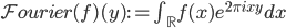
as the sequence of operations: First pull back f, i.e. consider it as a function in 2 variables. Then tensor it with something, i.e. multiply it with the kernel. Then push it down on the y-coordinate, which is integration over the x-part. This can be said geometrically for a correspondence and leads directly to the Fourier-Mukai transform, which is "the Fourier transform for sheaves". This can be applied to prove the Geometric Langlands Correspondence in the n=1 case, where sheaves on $Pic(X)$ are considered. Classical Fourier transform works on a torus, and in the complex analytic topology, $Pic(X)$ is a torus. So the analogy should be clear.

The "right" choice of sheaves for the Geometric Langlands Correspondence are now certain perverse sheaves. Perverse sheaves, because they enjoy Verdier duality, a relative version of Poincaré duality and certainly a powerful tool. The "certain" means "Hecke eigensheaves" which I don't want to explain for now. And, of course, I don't want to even try to explain what perverse sheaves on a stack are, since I have no idea. The same applies to the L-function side of the story.

Geometric Langlands Correspondence

To summarize, the correspondence says, for a smooth projective curve $X$ over $\mathbb{F}_q$ or $\mathbb{C}$, the n-dimensional local systems correspond 1:1 to the Hecke eigensheaves, certain perverse sheaves on the moduli stack of n-dimensional vector bundles.

$$Loc^n(X) \leftrightarrow \text{Hecke-Eigensheaves in } Perv(Bun_n(X))$$

There are more translations to be made, for example we can replace the perverse sheaves with D-modules when working over $\mathbb{C}$, which might be more natural to understand at first sight (since we replaced "representations in automorphic functions" with "systems of differential equations" which you can think of as modelling the space of functions as solution space).

In the $n=1$-case, the whole business is strongly related to the Fourier-Mukai transform and in general, somewhere is physics involved in more conjectures on the whole setup. I am unable to comment on that, but if you're interested, the article of Frenkel (did I mention that?) is a good point to start reading.

Maybe I should also mention that the whole thing can be done for any reductive group instead of $GL_n$, but then there are no proofs, only conjectures. Also, in the ramified case, a conjecture can be made but it is not proved even for $GL_n$.